
Students working together on a lab activity.
Structural Geology Lab, 2021
This page is (always) under construction
You can submit paper copies of your work directly to Professor Cronin.
Instructions for how to submit your lab work digitally are provided in the web document "Assignment Submittal Instructions" accessible via Assignment-Submit-Instructions.html
Lab 1: Some math basics
- Sig figs, rounding, and simple counting statistics -- Excerpt2-Lab1-AGILM.pdf
Example of an Excel spreadsheet for computing some simple counting statistics: SimpleCountingStatistics.xlsx
Assignment 1 — Worksheet on simple counting statistics: CountingStatisticsWorksheet.docx
-
Basics of vectors and vector arithmetic --
VectorSummary.pdf
Assignment 2 — Worksheet on vectors:
VectorWorksheet.pdf
Lab 2: More math basics
-
Introduction to matrices --
Matrices.pdf
Assignment 3 Worksheet on matrices:
matrix_dot_product_worksheet.v2.pdf
-
Orthogonal coordinate transformations --
OrthogonalCoordTrans.pdf
Assignment 4 Worksheet on coordinate transformations:
CoordTransHW.pdf
-
Using spreadsheets to solve common types of problems; examples
-
Bearing.xls
-
CrossProduct.xls
-
FindDecimalDegrees.xls
-
FindLatAndLong.xls
-
FindLocationVector.xls
Lab 3: Intro to determining crustal strain from GPS velocities
A good online source of information about GPS technology and its use in geoscience is the UNAVCO Spotlight site accessible via
https://spotlight.unavco.org
.
-
Student resources for GETSI module "GPS, Strain, and Earthquakes":
serc.carleton.edu/s/getsi/gps_strain/index.html
-
Background information about GPS/GNSS technology and its application in geoscience:
https://spotlight.unavco.org
-
What can GPS tell us about future earthquakes?
https://www.iris.edu/hq/inclass/animation/pacific_northwest_vs_japan_similar_tectonic_settings
or, for a direct download,
https://www.unavco.org/education/outreach/animations/Japan-vs-PacificNW_What-can-GPS-tell-us.mp4
-
Sendai/Tohoku-oki earthquake displacements using 1 Hz data (by Ronni Grapenthin):
https://youtu.be/rMhhyb6Yy94
-
GPS as an essential component of Cascadia earthquake early warning:
https://www.iris.edu/hq/inclass/animation/earthquake_early_warning_pacific_northwest_subduction_zone
or, for a direct download,
https://www.unavco.org/education/outreach/animations/GPSEarthquakeEarlyWarning.mp4
- The primer on instantaneous strain in 1D, 2D, and 3D can be downloaded from https://croninprojects.org/Vince/Geodesy/GPS_Strain_Primer.doc
- The "homework" worksheet is available at https://croninprojects.org/Vince/Course/IntroStructGeol/ExtensionWorksheetV2.pdf
- The web pages associated with that worksheet begin at https://croninprojects.org/Vince/PhysModel/1D_1.html
- The video showing the GPS strain analysis of three sites just west of Portland in Cascadia is on YouTube at https://youtu.be/gNGs7oW9aAU
- The video showing a simple visualization of a GPS strain analysis is on YouTube at https://youtu.be/HGnr4dSE92I
- Some web pages showing the construction of the "stretchy cloth" strain model I demonstrated begin at https://croninprojects.org/Vince/PhysModel/1D_1.html
- Nicky Arellano's video about making the stretchy-cloth model is accessible via https://croninprojects.org/Vince/PhysModel/Uniax2D_def.html. The video is also available on YouTube at https://youtu.be/mS5-X5N0pvE
- Remember that rigid-body deformation = translation + rotation
- Remember that non-rigid-body deformation = translation + rotation + volume strain (dilation) + distortion (change of shape)
- positive rotation is anti-clockwise (right-handed rotation)
- positive dilation is an increase in volume
- Remember that stretch = 1 + elongation, where a positive elongation is an increase in final length relative to the original length.
- Physical models of Earth structures:
PhysModelAnimations.html
and
https://croninprojects.org/Vince/PhysModel/
-
Images of different strain scenarios for triangles:
https://croninprojects.org/GETSI-EER2018/gps_triangle_strain_ellipse.pdf
(pdf, 1.8 MB) [
Microsoft Word .docx file, 1.8 MB
]
Lab 4: Doing the crustal strain analysis using GPS velocities
- Different triangle-strain scenarios: https://croninprojects.org/GETSI-EER2018/gps_triangle_strain_ellipse.pdf
- Video "How to find GPS velocity data from UNAVCO station overview pages": https://youtu.be/BYzCZh3RpyU
- NOTA GNSS/GPS Stations Network Monitoring
https://www.unavco.org/instrumentation/networks/status/nota/gps
-
Interactive PBO GPS network map:
https://www.unavco.org/instrumentation/networks/status/pbo/gps
-
Cascadia example worksheets:
https://croninprojects.org/GETSI-EER2018/Cascadia-Example.pdf
(.pdf file 2 MB) [
Microsoft Word .docx file, 2 MB
] -->
-
Generic datasheet for velocity data from 3 GPS/GNSS sites:
https://croninprojects.org/Vince/Geodesy/GPS-strain-datasheet.pdf
(pdf file, 125.8 kb)
-
GPS strain Calculators
-
How to interpret the strain calculator output:
https://d32ogoqmya1dw8.cloudfront.net/files/getsi/teaching_materials/gps_strain/explanation_gps_strain_calculator.v3.pdf
(.pdf file) [
Microsoft Word .docx file
]
-
Strain ellipse visualization tool (
https://d32ogoqmya1dw8.cloudfront.net/files/getsi/teaching_materials/gps_strain/strain_ellipse_visualization_t.zip
), which requires a free copy of Wolfram CDF Player (
https://www.wolfram.com/cdf-player/
)
- Cascadia example recap: https://youtu.be/gNGs7oW9aAU
-
Background information
Lab 5: Assignment due Wednesday September 29
Assignment 5 Complete an instantaneous/infinitesimal-crustal-strain analysis of the triangle of crust between GNSS/GPS stations P146, P149, and P150, located near Stampede Reservoir (just north of Lake Tahoe).
- Download a copy of the generic datasheet: https://croninprojects.org/Vince/Geodesy/GPS-strain-datasheet.pdf
- Go to the NOTA GNSS/GPS Stations Network Monitoring site: https://www.unavco.org/instrumentation/networks/status/nota/gps
- Either use the map or scroll through the table below the map to find Site P146, then click on the blue P146 link.
- On the P146 - Overview/Station Page, find the box labeled "Station Data," then the item "Time Series Data," then click on the "NAM14_CSV" link to go to the CSV (comma separated values) file that lists data for P146 in the North American Datum of 2014.
Note that there is a video titled "How to find GPS velocity data from UNAVCO station overview pages" that is accessible via https://youtu.be/BYzCZh3RpyU
- In the 11th line from the top of the header of the CSV file -- the line that starts with "Reference position" -- find the latitude and longitude data and copy those coordinates onto your generic data sheet.
- Return to the P146 - Overview/Station Page and locate the graphic under the heading "Station Position," and click on the graphic. It will expand into a full-size page. Use the navigation arrow on the right side of the window to get to the third page of time-series graphs -- the one that includes the velocity and standard deviation above each of the time-series graphs. Copy the north velocity and σ (standard deviation), and the east velocity and σ onto your generic data sheet.
- Move on to the P149 and P 150 Overview/Station Pages. The easiest way is to change the last several characters in the URL of the P146 overview page. So, for example,
https://www.unavco.org/instrumentation/networks/status/nota/overview/P146
would be changed to
https://www.unavco.org/instrumentation/networks/status/nota/overview/P149
to allow you to access the P149 - Overview/Station Page.
- When you have all of the input data recorded on your generic data sheet, open the GPS Strain Calculator in Excel (or one of the other calculators) and input your data. The Excel version is available at https://CroninProjects.org/Vince/Geodesy/Calculators/GPS-strain-calculator-20210922.xlsx
(Excel 37 kb), and a related video is available at https://youtu.be/nJJudaorc4w.
- After all of the new data is input to the strain calculator, it will generate results. Copy those results onto your generic data sheet, and work on trying to understand their meaning.
- Compare your results with the other members of the class. Identify and resolve any discrepancies.
- Transcribe all of the data (input & output) onto a nice clean copy of the generic data sheet and bring it with you to lab on September 29.
Lab 6: Looking at crustal strain in different structural environments.
Assignment 6a Use GPS site velocities to characterize the crustal strain in the area between the triplet of GPS sites indicated below. Follow the general instructions given in lab 5, and submit the data sheet and Excel spreadsheet for each GPS triplet.
- AC26, AC34, AC39
- P538, P539, P541
- P088, P116, COON
Assignment 6b The link for the Quaternary Fault and Fold Database of the United States is https://www.usgs.gov/natural-hazards/earthquake-hazards/faults and, once there, work with their "Interactive Map.". How would you describe the active faults in the area near each of the crustal triangles we have investigated?
Lab 7: Some basic map skills
- Presentation on mapping topographic surfaces:
PDF version
or
Keynote version
- Access to USGS topographic maps in digital form via TopoView: https://ngmdb.usgs.gov/topoview/viewer/
-
Another source of GeoPDF files of USGS topographic maps:
viewer.nationalmap.gov/basic/?basemap=b1&category=ustopo&title=US Topo Download
- Link to the 2018 Cajon, California topographic map in JPEG file form (7.5 MB). Also available in KMZ, GeoTiff, and GeoPDF formats from TopoView
- UNAVCO video about LiDAR: https://youtu.be/chSywRqgIGY?list=PLzmugeDoplFM5pPI80wwi3qmtZH99Ism2
- NEON video about LiDAR: https://www.youtube.com/watch?v=EYbhNSUnIdU&feature=youtu.be
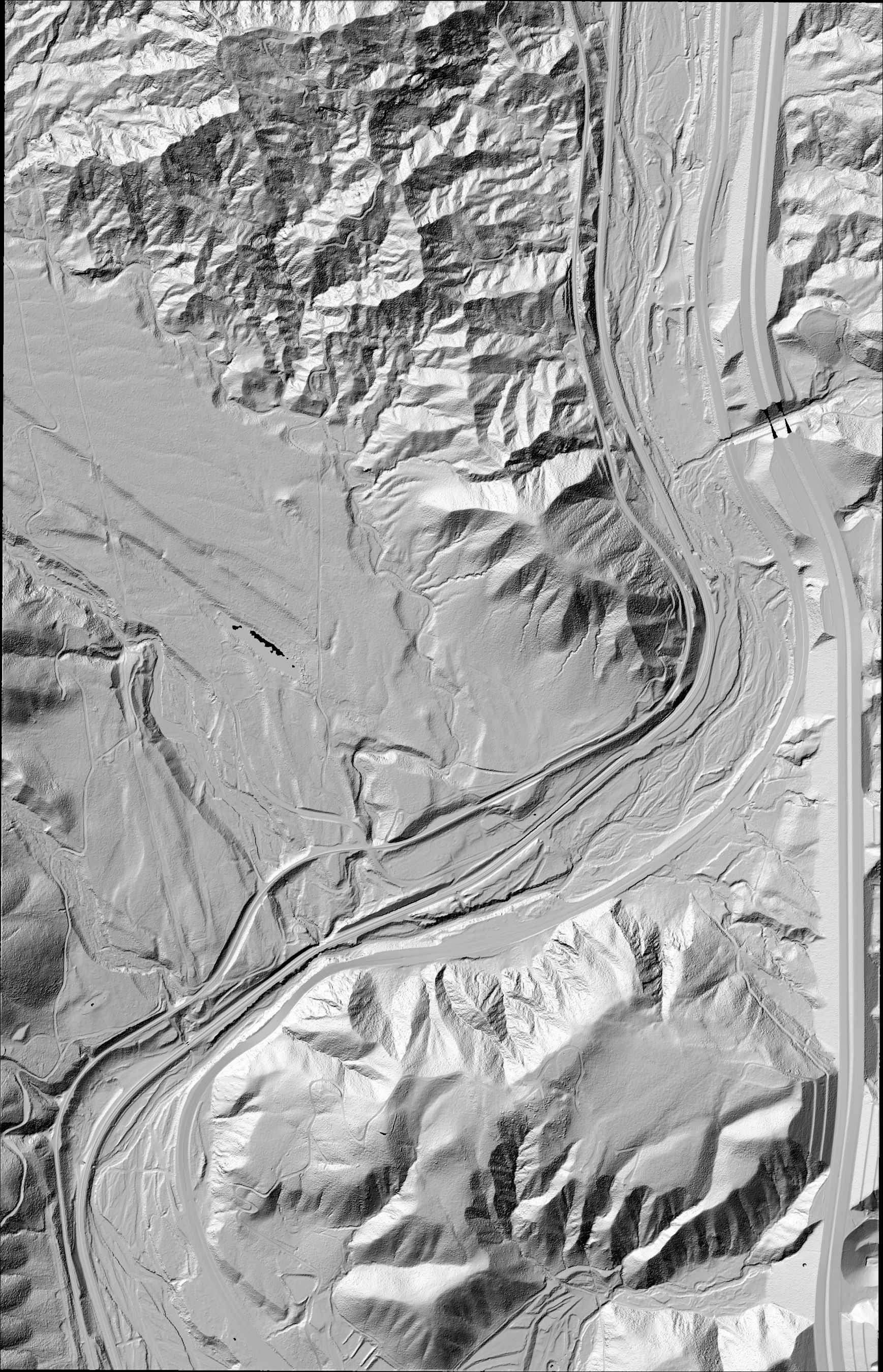
- Hillshade map of part of the southern Cajon Pass, California, made from LiDAR data at a resolution of 1 meter: https://CroninProjects.org/Vince/Course/IntroStructGeol/SouthernCajonPass.jpg. Data from https://OpenTopography.org
- Assignments to be completed and submitted via Canvas. Please label the elevation on each contour, and remember to put your name on anything you submit.
- Assignment 7 -- a random array of points: ContourMap-1.pdf
- Assignment 8 -- a gridded array of points: ContourMap-2.pdf
- Assignment 9 -- another random array of points: SimpleContouringExercise.pdf
- Assignment 10 Basic topo map interpretations and measurements: TopoMapExercise-1.pdf
View the video "Measuring distance using a bar scale" on YouTube at https://youtu.be/e62xi7IaBrU
Lab 8: Some ways of looking at a fault
Assignment 11 Record your responses on the activity sheet for lab 8, which is accessible HERE.
Remember that you have access to Microsoft 365 and, hence, to Microsoft Word as a Baylor student.
- View Dave McConnell's video "Classification of Faults" on YouTube at https://youtu.be/qlk7IfYMufs
- In Google Earth Pro (https://www.google.com/earth/versions/#earth-pro),
search for "Wallace Creek, Elkhorn Road, Santa Margarita, California"
- Look at the ground surface from eye altitudes of 1 to 10 km
- Note the latitude and longitude of the middle of the part of Wallace Creek that flows NW along some sort of linear feature. Do that by putting the cursor in the middle of that part of the stream channel and then reading the latitude and longitude in the footer along the lower right edge of the window.
If you need to re-set your app so it displays decimal latitudes and longitudes (i.e., so it looks like "lat 35.217...°" rather than "lat 35° 16'..."),
- go to the Google Earth Pro drop-down menu along the header bar of your screen,
- select "Preferences"
- in the "3D View" submenu, select "Decimal Degrees"
- Go to the TopoView map viewer (https://ngmdb.usgs.gov/topoview/viewer/) to find the topo map that includes Wallace Creek.
- In the dark gray box to the right of the window, select (i.e., click on) "24K" because we are looking for a 1:24,000 scale map
- Move the date slider on the left toward the right so that we are just looking for maps published recently -- since about 2010.
- Navigate to the California coastline between San Francisco and Los Angeles, and find San Luis Obispo. You will need to zoom in using the + button until you can see this town.
- From San Luis Obispo, scroll east (right) to McKittrick Summit.
- Center the McKittrick Summit quadrangle on your screen, and zoom in until it is the only thing on your screen. Click on the McKittric Summit quadrangle on your screen to select it.
- You will now see your map choices in the dark gray box to the right. Select (i.e., click on) "McKittrick Summit, CA 2018 (US Topo) Scale 1:24000"
- You now have several options for downloading digital map products. Download "GeoPDF (48 MB)"
- Open the GeoPDF.
- Along the left margin of the window is an icon that looks like a stack of papers.
- Click on this icon to view the map layers that are available in this GeoPDF file.
- Click in the square box next to the Images file folder to select it. An aerial photo image of this map area should now appear.
- Click on the ">" symbol to the left of the Map Frame folder to view its subfolders and files
- Deselect the Boundaries, Transportation, and Terrain folders to declutter the map.
- The UTM zone for this area is identified in the text in the lower left corner of the "collar" or border around the map. It consists of a number and a capital letter.
- The yellow grid marks the UTM grid for this map area. The numbers from 39 to 49 along the bottom of the map indicate the UTM eastings, and the numbers from 05 to 18 along the sides of the map indicate the UTM northings. The full easting is printed for one of the eastings at the lower right and upper left corners of the map — for example, 249,000mE, with the "49" printed larger than the other numbers. Similarly, the full northing for one of the northings is printed in the lower right and upper left corners of the map — for example, 3918000mN, with the "18" printed larger than the other numbers. Each of the grid boxes is 1000 meters on a side (one square kilometer).
- Find the grid box between 242000mE and 243000mE, and between 3906000mN and 3907000mN.
- Expand it as much as you can on your screen, then make a screen grab and print the result so you are working from a paper map.
- Using the yellow grid lines as your scale, what is a higher-resolution set of UTM coordinates for the middle of the active channel of Wallace Creek where its active main channel coincides with the San Andreas fault trace?
- With the UTM box containing Wallace Creek still centered on your screen, turn off (deselect) the Image layer and turn on (select) the Terrain layer, so the result is that you are looking at topographic contours and the yellow UTM grid. Could you have located the place where Wallace Creek is deflected along the San Andreas fault from these topographic lines alone? Explain your answer (how, why not, etc.).
- Now turn the Image layer back on so that there are topo lines on top of the aerial photo. How would you describe the apparent accuracy of the topographic contours on this map -- do they look like they are a true reflection of the shape of the ground surface?
- We now go in search of the interactive fault map that displays the Quaternary Fault and Fold Database of the United States. If you don't have the direct link (https://usgs.maps.arcgis.com/apps/webappviewer/index.html?id=5a6038b3a1684561a9b0aadf88412fcf), the easiest thing to do is search on these two terms (together): Faults USGS. That should get you to a list where you can find the following link: https://www.usgs.gov/natural-hazards/earthquake-hazards/faults
- Click on that link to get to a USGS page where you can click a link to the "Interactive fault map": https://doi.org/10.5066/F7S75FJM
https://usgs.maps.arcgis.com/apps/webappviewer/index.html?id=5a6038b3a1684561a9b0aadf88412fcf
- Once there (a map site run by esri), you can go to Select a Location box and enter San Luis Obispo, CA.
- Then bump the "—" button once or twice to get to a better "elevation" and scroll east to the boundary between Soda Lake on the Carrizo Plain and the Temblor Range. Zoom back in with the "+" button to find Wallace Creek. It won't be labeled, so you will just have to compare what you see with your acquired knowledge of what Wallace Creek looks like, with its deflected stream course. Notice the colors of the various fault strands. Click on them to see how they are described (if they are described at all, that is...).
- When the "click for a description" function does work, it gives you access to a description of the Cholame-Carrizo section of the San Andreas fault, which is also accessible directly via https://earthquake.usgs.gov/cfusion/qfault/show_report_AB_archive.cfm?fault_id=1§ion_id=g
- For the following steps, it is suggested that you use either Firefox, Chrome, "or another WebGL2 browser" so that you will have full access to the results.
- Go to OpenTopography.org (https://opentopography.org/) and sign-in using your Baylor email address (or register if you have not already done so).
- Once you are in OpenTopography, use the DATA drop-down menu to select FIND DATA MAP.
- Use the "+" button to magnify, and drag the map so that you are eventually looking at the San Andreas fault area near Wallace Creek, California. Remember from previous steps that it is east of San Luis Obispo, and is along the west side of the Temblor Range. As you zoom in, you will be focused on the red strip along the west edge of the Temblor Range on the east side of the Carrizo Plain, near the boundary between Kern and San Luis Obispo Counties. Click on that red strip near where you think Wallace Creek is located.
- A box should appear that provides the following information:
Dataset Name: B4 Project - Southern San Andreas and San Jacinto Faults
The dataset name is a link to the dataset, so click on that link.
- A new window will open with information about the B4 project and its data. Click on the blue button labeled Point Cloud Data
- In the next window, scroll down to "1. Coordinates & Classification" and make exactly the same choices as shown in the screen-captured image "WallaceCreekDetailSpecs.pdf".
- In the "Job Description" part of the form, give your job a name and a brief description where prompted, and enter your email address.
- Check to be sure all of the input is correct (all of the right boxes are selected or deselected, all of the input numbers and choices are correct, the job description is complete) and then click the blue SUBMIT button.
- You can then wait a few minutes for the job to complete, or check your email later for a link to the results.
- Download the DEM Results (a file called "output.tin.tar.gz") and the hillshade map from the "Visualization Products" area of the job results. On a Mac, I press the control key and click the image, then choose "Download Linked File," or open the file by clicking on it, then press the control key, click the enlarged image, and choose "Save Image As..." On a Windows machine, the equivalent might be to right-click the image and save it to your computer. Either way, the file name should be "viz.tin.hs.white.png."
- Click on the "output.tin.tar" file on your computer to decompress it, resulting in another file called "output.tin.asc."
Open this file with a text editor such as TextEdit or BBEdit or just about any other generic text editor. What you will see is six header rows that specify various important information about the datafile (number of columns, number of rows, the UTM coordinates of the lower left corner of the dataset, the horizontal spacing between nodes in the square grid, and the value used to indicate a missing value in the dataset), followed by hundreds or thousands of rows and columns of data. Each datum in that sea of numbers is an elevation above sea level.
It is this dataset of elevations that allows us to write computer code to analyze or visualize the ground surface in this area. How to do that is a topic for another time.
- Note the following videos that should fortify and extend what you have just done:
- Geographic2UTM conversion using NCAT: https://youtu.be/1l4NJNpBJKQ
- Getting a DTM and hillshade map from OpenTopography.org: https://youtu.be/hcRqC2bYS14
- Using the research code Hillshade-2020.nb in Mathematica: https://youtu.be/4zEVmCVqJGI
Lab 9: Orientation measurements, and the Brunton compass
Some items related to faults
An oral presentation was made at our meeting on October 27 that referred to a set of slides. They are available below in several formats:
Strike and dip of a surface
Definitions
The azimuth of a horizontal line or line segment is determined on a horizontal plane, measured clockwise from true north. Azimuths range from 0 to 360°. So, for example, a horizontal vector pointing due east has an azimuth of 90°.
The strike of a surface at a given point is the azimuth of a horizontal line tangent to that surface at that point.
The dip vector of a surface at a given point is a unit vector tangent to the surface at that point that is oriented in the direction of steepest descent on that tangent plane. It is the direction that a ball would roll down the tangent plane.
The dip angle of a surface at a given point is the angle between the dip vector and a horizontal plane that is measured in the vertical plane that contains the dip vector. The dip angle is the same as the plunge of the dip vector. The dip angle ranges from 0° (horizontal) to 90° (vertical).
The dip direction of a surface at a given point is indicated by the vertical projection of the dip vector onto a horizontal plane. The dip direction might be expressed as an azimuth or it might be informally indicated by directional descriptions (N, NE, E, SE, S, SW, W, NW). When expressed as an azimuth, the dip direction is the same as the trend of the dip vector.
Geologists describe the orientation of a surface at a given point using three bits of information. There are several ways of doing this, including the following:
- Azimuth Method: strike azimuth (0-360°), dip angle (0-90°), and dip direction (N, NE, E, SE, S, SW, W, NW).
Example: the orientation of a plane striking 132° and dipping 48° toward the SW would be recorded as 132, 48SW. That is equivalent to 312, 48SW because 312° is 180° from 132°. The azimuth of either direction along the strike line is acceptable.
- Right-Hand Rule Method (RHR): explicit use of the right-hand-rule convention, strike azimuth (0-360°), dip angle (0-90°).
In this case, the dip direction is understood to be the strike azimuth + 90°. The RHR strike direction is based on the dip direction (the azimuth of the horizontal projection of the dip vector), in that the RHR strike is Example: the orientation of a plane striking 58° and dipping 76° (toward the SE) would be recorded using the right-hand-rule (RHR) as 58, 76.
- Quadrant Method: I do not teach this method because it is so error-prone.
That said, you should be able to convert from the quadrant method to the azimuth method, so some knowledge of the quadrant method (QM) is needed. All strike directions are measured relative to north.
- If the strike is 32° to the west of north, it is written "N32W" in the QM, which is equivalent to an azimuth of 360° – 32° = 328°.
- If the strike is 56° to the east of north, it is written "N56E" in the QM, which is equivalent to an azimuth of 56°.
- If the strike is 90° from N, there are a variety of options. The strike could be described as EW, due east, due west, N90E, N90W.
All dip angles and dip directions are expressed as in the azimuth method.
Example: the orientation of a plane striking 104° or 284° as expressed in the azimuth method and dipping 48° toward the SW would be recorded as N76W,48SW.
- If the "strike and dip" methodology had not been developed by workers in the mining and quarrying trades hundreds (thousands?) of years ago, the three bits of information we would use to describe the orientation of a surface might be the three vector coordinates of the vector that is normal to (i.e., perpendicular to) the surface at the point where its orientation is being described.
Lab 10: Structural-geologic contouring and surface maps
- Finding faults using structural contour maps of a surface
- Assignment 12
First faulted subsurface map:
ContourMap4.pdf
- Assignment 13
Second faulted subsurface map:
ContourMap3.pdf
- Intersection of two surfaces
-
TraceContour.pdf
- 3-point problems
-
Explanation of simple 3-point problem:
3-point-problem-explanation.pdf
-
Example given only the location and elevation of points:
3-point_problem.pdf
- Assignment 14
3-point problem using topographic contours for elevation data:
3Point-Topo.pdf
-
Working with contacts, contact traces, and unit thickness using topographic maps
- Assignment 15
Analyzing a complicated-looking contact on a topographic map:
Inclined-contact-topo.pdf
- Assignment 16
Contacts of vertical, horizontal, and inclined planes depicted on a topographic map:
vertical-horizontal-inclined-planes.pdf
-
Explanation of how to determine the thickness of an inclined planar bed using topographic contours:
Thickness-explanation.pdf
- Assignment 17
Working with bed thickness using contacts of inclined beds on a topographic map:
thickness-topo.pdf
JPEGs of the assignment maps in a compressed (zip) file: Lab10docs.zip
Lab 11: Structural cross sections, part 1
Set of simple cross-section problems:
BasicCrossSections.pdf
Some other docs used in the lab presentation
Lab 12: Use of a Brunton Compass
- Use the NOAA Magnetic Field Calculator (https://www.ngdc.noaa.gov/geomag/calculators/magcalc.shtml) to determine the magnetic declination for the location where the Brunton compass will be used.
-
Basic measurement skills with a Brunton compass:
BruntonCompassBasics.html
- Tips on using a Brunton Compass: TipsOnUsingABruntonCompass.docx, or TipsOnUsingABruntonCompass.pdf
-
Manual for operating the Brunton Pocket Transit:
Brunton_Transit_Manual.pdf
Other files and resources
Relevant UNAVCO/IRIS animations and videos
-
UNAVCO videos on U-Tube:
https://www.youtube.com/user/unavcovideos
-
Animation-and-video homepage at UNAVCO:
https://www.unavco.org/education/outreach/animations/animations.html
-
Earthscope's geodetic component -- Plate Boundary Observatory (PBO) overview:
https://youtu.be/EPlCcRFpTuU
-
GPS Measures Deformation in Subduction Zones: Ocean/continent:
https://www.iris.edu/hq/inclass/animation/gps_measures_deformation_in_subduction_zones_oceancontinent
or, for direct download,
https://www.iris.edu/hq/inclass/downloads/download/95
-
GPS Measures Deformation in Subduction Zone: Island Arc Setting:
https://www.iris.edu/hq/inclass/animation/gps_measures_deformation_in_subduction_zone_island_arc_setting
or, for direct download,
https://www.iris.edu/hq/inclass/downloads/download/96
-
GPS Records Variable Deformation across a Subduction Zone:
https://www.iris.edu/hq/inclass/animation/gps_records_variable_deformation_across_a_subduction_zone
or, for direct download,
https://www.iris.edu/hq/inclass/downloads/download/92
-
What can GPS tell us about future earthquakes?
https://www.iris.edu/hq/inclass/animation/pacific_northwest_vs_japan_similar_tectonic_settings
or, for a direct download,
https://www.unavco.org/education/outreach/animations/Japan-vs-PacificNW_What-can-GPS-tell-us.mp4
-
Sendai/Tohoku-oki earthquake displacements using 1 Hz data (by Ronni Grapenthin):
https://youtu.be/rMhhyb6Yy94
-
GPS as an essential component of Cascadia earthquake early warning:
https://www.iris.edu/hq/inclass/animation/earthquake_early_warning_pacific_northwest_subduction_zone
or, for a direct download,
https://www.unavco.org/education/outreach/animations/GPSEarthquakeEarlyWarning.mp4
-
ShakeAlert: Earthquake Early Warning System for Napa earthquake 2014:
https://www.iris.edu/hq/inclass/animation/shakealert_earthquake_early_warning_system
or, for direct download,
https://www.iris.edu/hq/inclass/downloads/download/407
-
Basin & Range: GPS measures extension:
https://www.iris.edu/hq/inclass/animation/basin__range_gps_measures_extension
or, for direct download,
https://www.iris.edu/hq/inclass/downloads/download/193
-
Tectonics & Earthquakes of the Himalaya:
https://www.iris.edu/hq/inclass/animation/tectonics__earthquakes_of_the_himalaya
or, for direct download,
https://www.iris.edu/hq/inclass/downloads/download/466
-
Volcano Monitoring: Measuring Deformation and Tilt with GPS:
https://www.iris.edu/hq/inclass/animation/volcano_monitoring_measuring_deformation_and_tilt_with_gps
or, for direct download,
https://www.iris.edu/hq/inclass/downloads/download/138
-
Glaciers are retreating. How can we measure the full ice loss?
https://youtu.be/FVm3rZZs49s?list=PLzmugeDoplFOot41MIBBZiLYBCB0M-p1P
-
Plate tectonics 540Ma to the modern world, from Chris Scotese:
https://youtu.be/g_iEWvtKcuQ
-
Plate tectonics 240Ma to 250 million years in the future, from Chris Scotese:
https://youtu.be/uLahVJNnoZ4
If you have any questions or comments about this site or its contents, drop an email to the humble
webmaster
.