
A sunset view of Stampede Reservoir taken at low water level, summer 2016. Stampede dam is in the lower right corner.. Photo by Vince Cronin.
Hobart et alia Presentation for GSA Annual Meeting 2020
This page is in draft form and is subject to revision.
Reload this page in your browser every time you visit this page to be certain that you are reading the most current course information
------------------------------------oOo------------------------------------
Citation
Hobart, Catherine, Dunbar, J., White, J., and Cronin, V.S., 2020, A preliminary look at whether activity on the Polaris Fault could increase the potential for activity on the Dog Valley Fault near Truckee, California: Geological Society of America, Abstracts with Programs, v. 52, no. 6, doi: 10.1130/abs/2020AM-356509, https://gsa.confex.com/gsa/2020AM/meetingapp.cgi/Paper/356509
Corresponding Author: Catherine Hobart, who is accessible via Kate_Hobart1@baylor.edu
About The Author
|
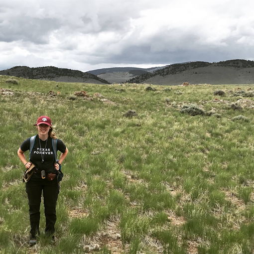
I am a second-year Master of Science (MS) student in the Geosciences Department at Baylor University. I graduated Magna Cum Laude with a Bachelor of Science (BS) degree in Geology from Texas A&M University, with a minor in Geographic Information Systems (GIS).
I have worked on a number of research projects, including two undergraduate planetary geology projects and my current MS thesis on the Dog Valley Fault. I have diverse internship experience, including two engineering internships with the National Aeronautics and Space Administration (NASA) and one internship with RPS North America, a global consulting firm focused on energy and resources.
I will be taking the Geologist-In-Training (GIT) Certification test in March 2021 and graduating in May 2021. I plan to pursue a career in Engineering Geology. |
A resume and other data are available upon request: Kate_Hobart1@baylor.edu
Abstract
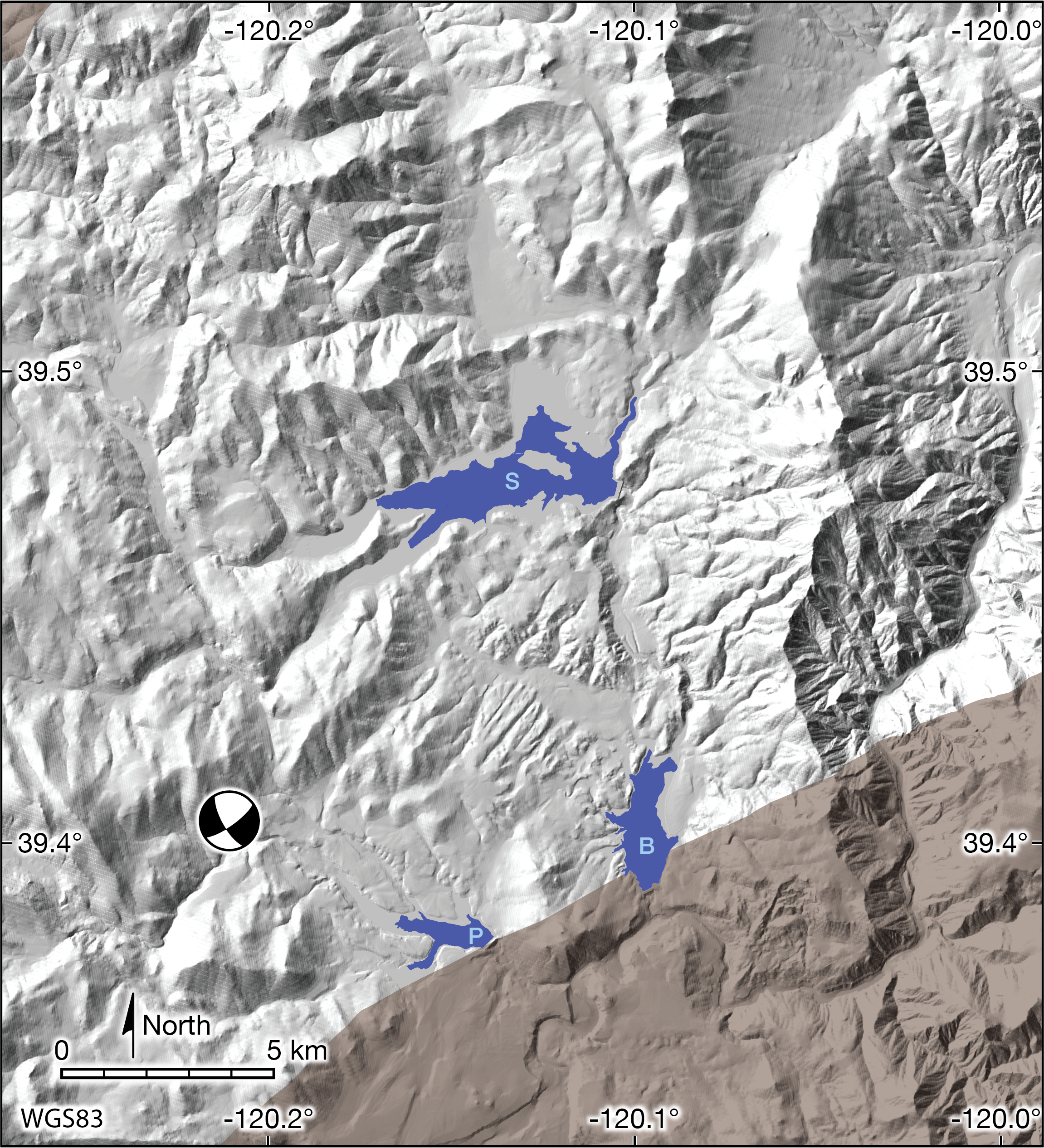
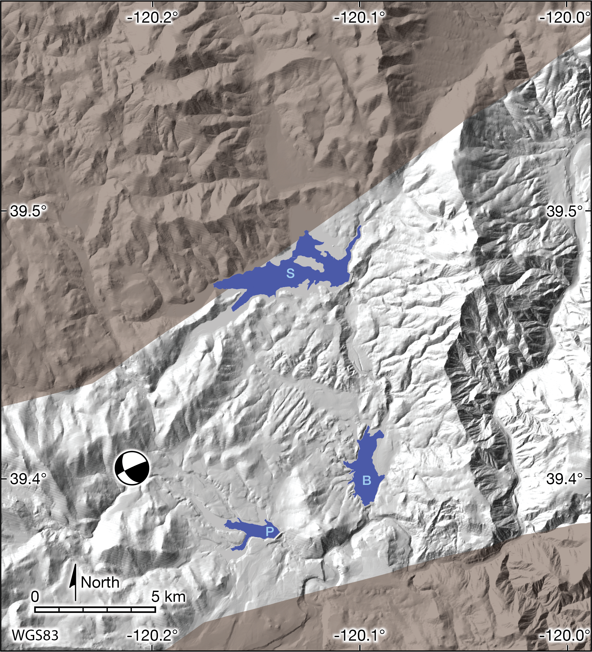
A fundamental goal of Engineering Geoscience is to recognize geologic hazards and work with society to avoid or mitigate risk from those hazards. In 1966, the Dog Valley Fault (DVF) near Truckee, California, generated a M6 earthquake, prior to the completion of Stampede Dam by the US Bureau of Reclamation in 1970. Although some geomorphic evidence exists in the area of the DVF, its coherent ground-surface trace remains uncertain to this day. Similar magnitude future earthquakes along the DVF could endanger Prosser Creek Dam, Boca Dam, and Stampede Dam, which lies perhaps on or nearly adjacent to the DVF trace (USBR, 2012, p. B14-B15). More recently, the nearby, NW-trending Polaris fault (PF), which can be considered a SE extension of the Mohawk Valley fault zone along the SW boundary of the northern Walker Lane shear zone, was recognized and judged to be an active right-lateral fault. The PF is capable of generating earthquakes in the M6-7 range that could endanger the earth-fill dams along Martis Creek and Prosser Creek (Hunter et al., 2011, BSSA v. 101, 1162). Water and debris from failed dams in this area would flow down the Truckee River and into Reno, Nevada, potentially causing damage and human casualties.
Based on our preliminary analysis using hillshade images made from a lidar-based DEM at 1 m resolution, the DVF is interpreted to intersect or perhaps cross the PF. Slip on one structure could result in significant stress changes and slip on the other, in a manner similar to the 2019 Ridgecrest and the 1987 Elmore Ranch-Superstition Hills earthquake sequences. Attempts to interpret the potential seismicity of the DVF as a singular, isolated structure without considering its structural context along with the active PF likely underestimates the hazard potential. Our objective is to conduct [1] seismo-lineament analysis and statistical best-fit-plane evaluation of relocated earthquakes and [2] structural-geomorphic analysis of hillshade maps created from lidar data. This analysis includes lineament mapping with GIS-based techniques such as convolution filtering, drainage network analysis, and stream deflection mapping, augmented by additional soil survey and near infra-red vegetation data to identify possible faults. We will also use GPS-site velocity data to measure present-day crustal strain in the area of the DVF.
Abstract & Poster References
Ashburn, J.A., 2015, Investigation of a lineament that might mark the ground-surface trace of the Dog Valley Fault, Truckee area, northern California: Baylor University, B.S. thesis, available via http://CroninProjects.org/Vince/AshburnBSThesis2015.pdf.
Fielding, E.J., Liu, Z, Stephenson, O.L., Zhong, M., Liang, C., Moore, A., Yun, S-H., and Simons, M., 2020, Surface deformation related to the 2019 Mw 7.1 and 6.4 Ridgecrest Earthquake in California from GPS, SAR Interferometry, and SAR Pixel Offsets: Seismological Research Letters, v. XIX, no. XX, p. 1-12.
Greensfelder, R., 1968, Aftershocks of the Truckee, California earthquake of September 12, 1966: Bulletin of the Seismological Society of America, v. 58, no. 5, p. 1607- 1620.
Hunter, L.E., Howle, J.F., Rose, R.S., and Bawden, G.W., 2011, LiDAR-assisted identification of an active fault near Truckee, California: Bulletin of the Seismological Society of America, v. 101, no. 3, p., 1162-1181, doi:10.1785/0120090261.
OpenTopography.org, 2020, 2014 USFS Tahoe National Forest Lidar, 1-m DEM, https://doi.org/10.5069/G9V122Q1
Ryall, A., Van Wormer, J.D., and Jones, A.J., 1968, Triggering of micro-earthquakes by earth tides, and other features of the Truckee, California, earthquake sequence of September, 1966: Bulletin of the Seismological Society of America, v. 58, no. 1, p. 215-248.
Strasser, M.P., 2017, Spatial correlation of selected earthquakes with the Dog Vally Fault in northern California using LiDAR and GPS data: MS thesis, Baylor University, accessible via http://croninprojects.org/Strasser/Matthew_Strasser_Masters.pdf
Tsai, Y-B., and Aki, K., 1970, Source mechanism of the Truckee, California earthquake of September 12, 1966: Bulletin of the Seismological Society of America. v. 60, no. 4, p. 1199-1208.
Current Graphics Suitable for Inclusion in Thesis
Revised January 9, 2021
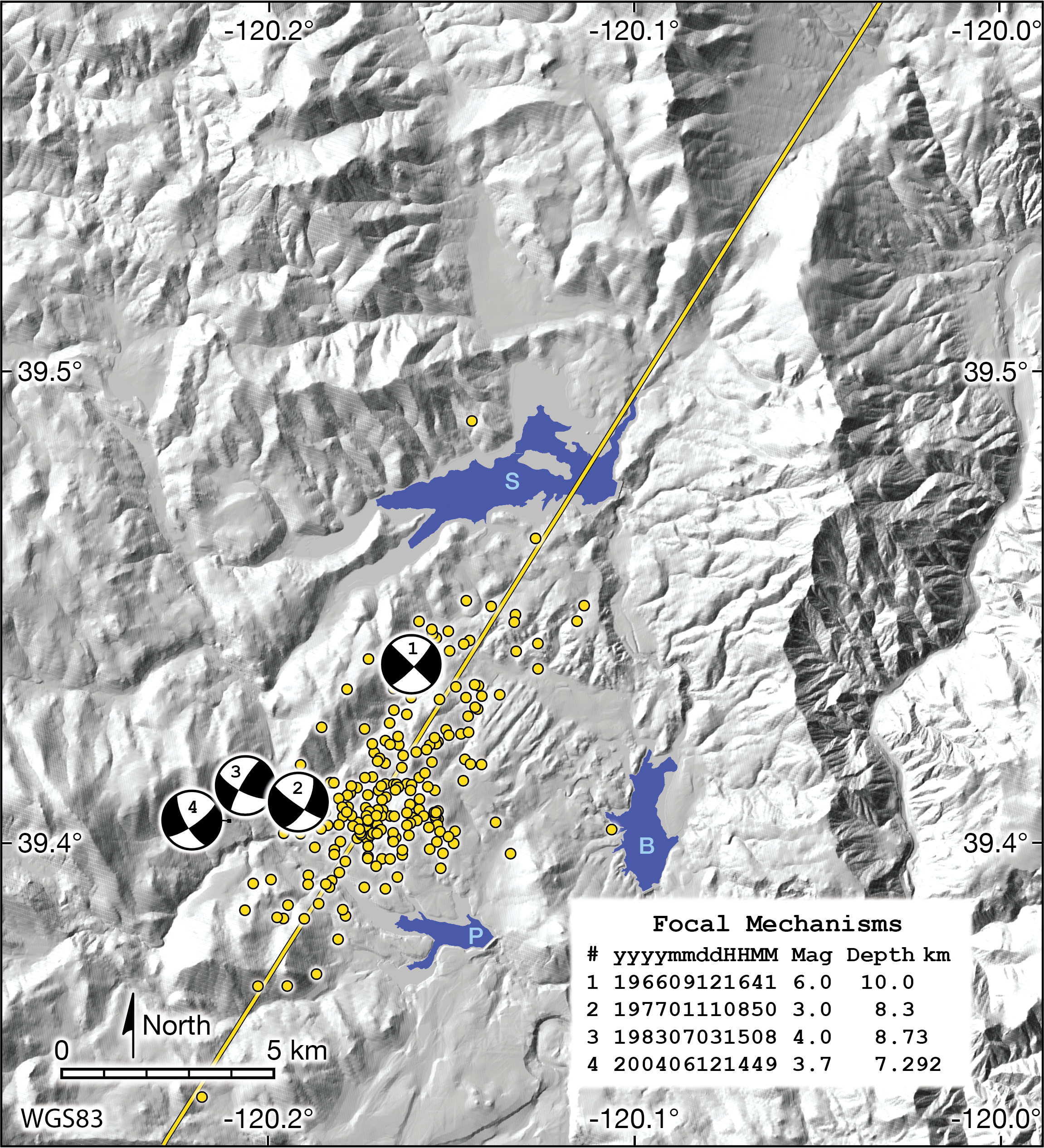
- Basemap plus focal mechanism for 1966 M6 earthquake: Map01_1966EQFM_2021Jan08.png
- Basemap, focal mechanism, and seismo-lineament for 1966 M6 earthquake: Map02_1966EQFMSL_2021Jan08.png
- Basemap plus focal mechanism for 1977 earthquake: Map03_1977EQFM_2021Jan08.png
- Basemap, focal mechanism, and seismo-lineament for 1977 earthquake: Map04_1977EQFMSL_2021Jan08.png
- Basemap plus focal mechanism for 1983 earthquake: Map05_1983EQFM_2021Jan08.png
- Basemap, focal mechanism, and seismo-lineament for 1983 earthquake: Map06_1983EQFMSL_2021Jan08.png
- Basemap plus focal mechanism for 2004 earthquake (21370352): Map07_2004EQFM_2021Jan08.png
- Basemap, focal mechanism, and seismo-lineament for 2004 earthquake (21370352): Map08_2004EQFMSL_2021Jan08.png
- Basemap plus focal mechanism for 2004 earthquake (21370353): Map09_2004EQFM_2021Jan08.png
- Basemap, focal mechanism, and seismo-lineament for 2004 earthquake (21370353): Map10_2004EQFMSL_2021Jan08.png
- Basemap plus focal mechanisms for 1966. 1977, 1983, and 2004 (21370352) earthquakes: Map11_FourEQFM_2021Jan08.png
- Basemap, focal mechanisms, and seismo-lineaments for 1966. 1977, 1983, and 2004 (21370352) earthquakes: Map12_FourEQFMSL_2021Jan08.png
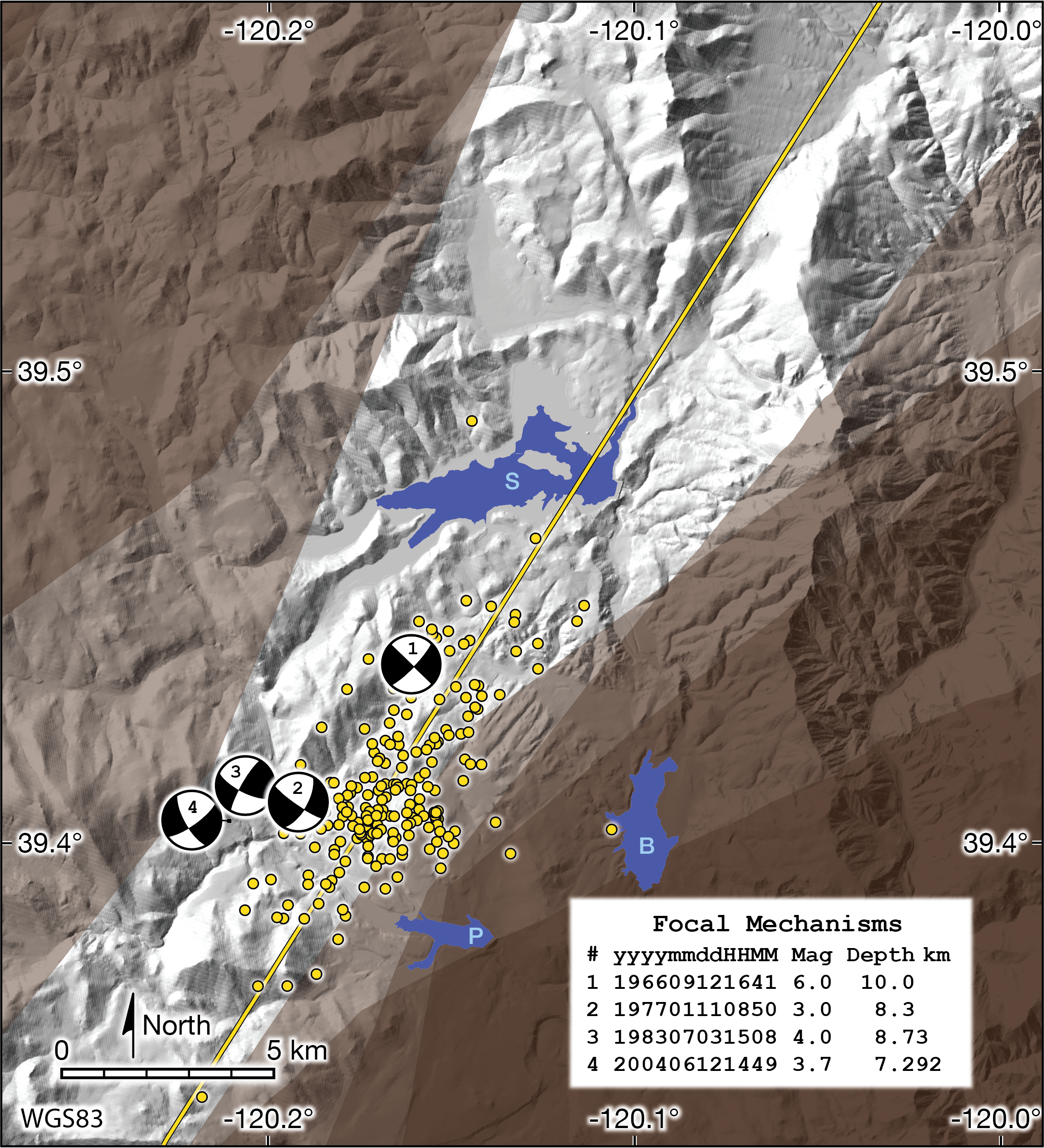
- Basemap, focal mechanisms for 1966. 1977, 1983, and 2004 (21370352) earthquakes, and aftershock epicenters: Map13_aftershocksAndFourEQFM_2021Jan08.png
- Basemap, aftershock epicenters, focal mechanisms and seismo-lineaments for 1966. 1977, 1983, and 2004 (21370352) earthquakes: Map14_aftershocksAndFourEQFMSL_2021Jan08.png
- Basemap, focal mechanisms for 1966. 1977, 1983, and 2004 (21370352) earthquakes, aftershock epicenters, and trace of best-fit plane through the aftershocks: Map15_aftershocksBFP_FourEQFM_2021Jan08.png
- Basemap, aftershock epicenters, focal mechanisms and seismo-lineaments for 1966. 1977, 1983, and 2004 (21370352) earthquakes, and trace of best-fit plane through the aftershocks: Map16_aftershocksBFP_FourEQFMSL_2021Jan08.png
Aftershocks and Best-Fit Plane Analysis
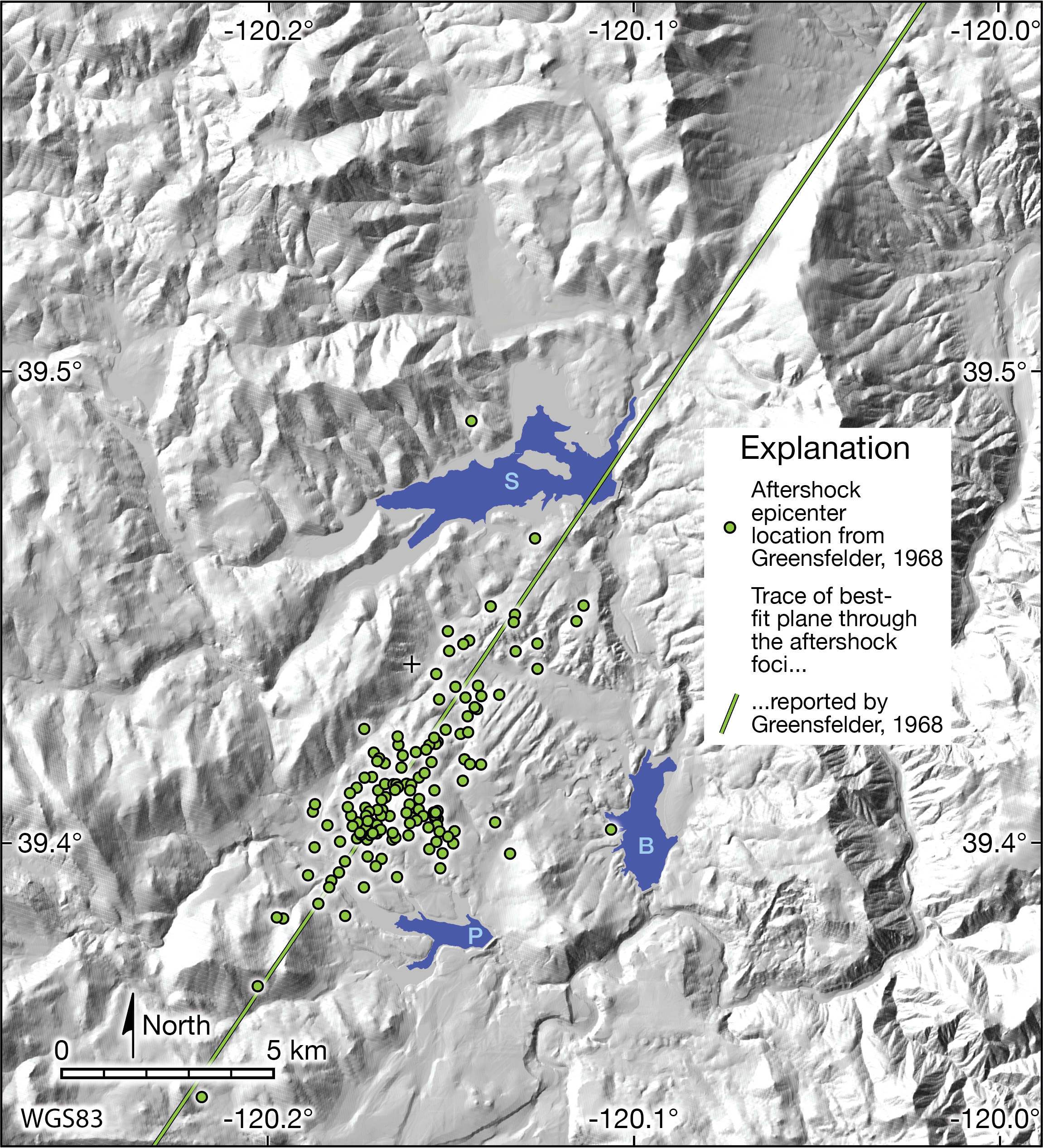
- Finished map from Adobe Illustrator file AftershocksBFPWGS83_Jan09.ai with aftershock epicenters from Greensfelder (1968): https://croninprojects.org/Hobart/Map17_GreensfelderAftershocks_V2.png
- Finished map from Adobe Illustrator file AftershocksBFPWGS83_Jan09.ai with aftershock epicenters from Greensfelder (1968) and the trace of the best-fit plane through those aftershock foci: https://croninprojects.org/Hobart/Map18_GreensfelderAftershocks&GBFP_V2.png
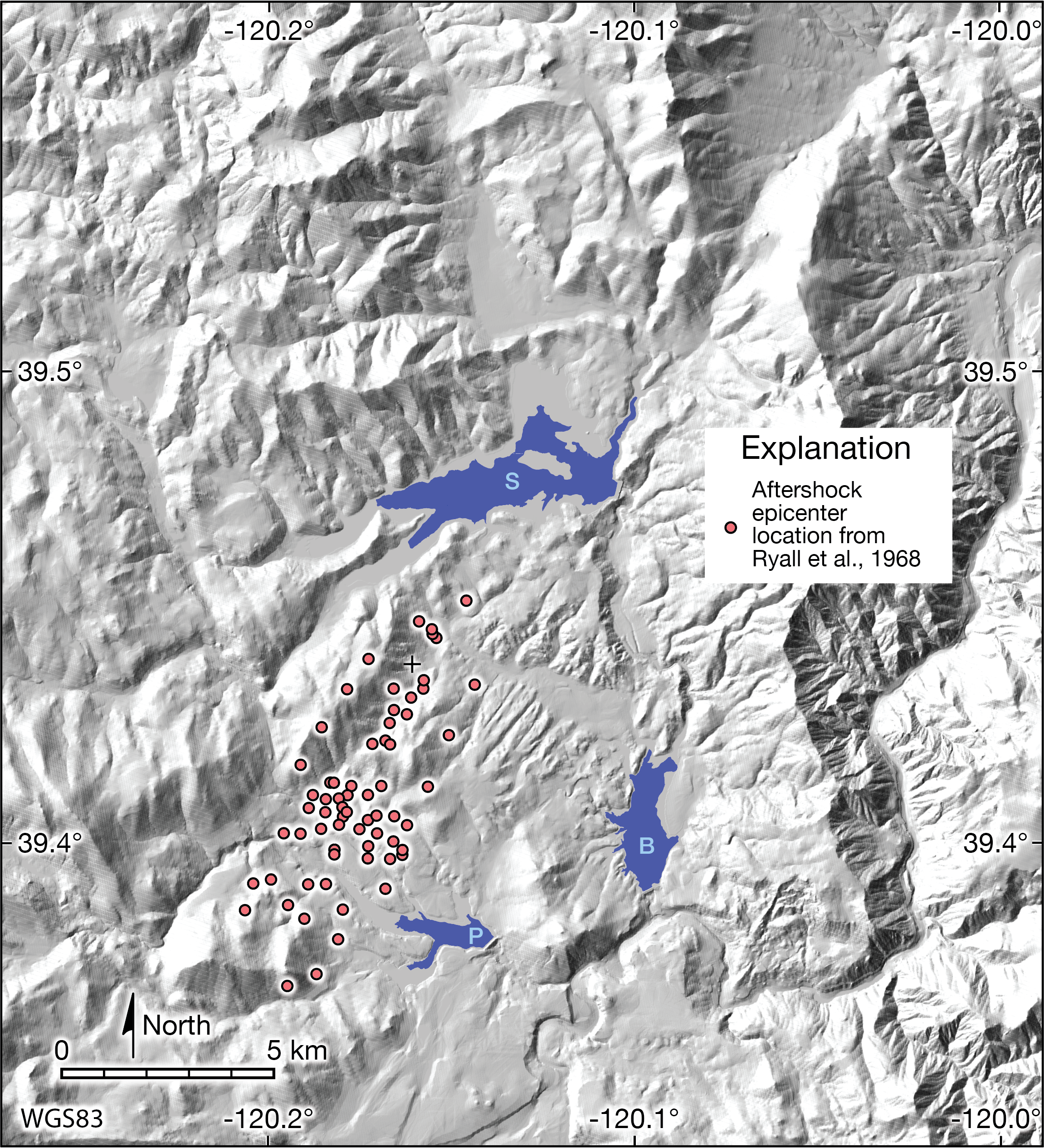
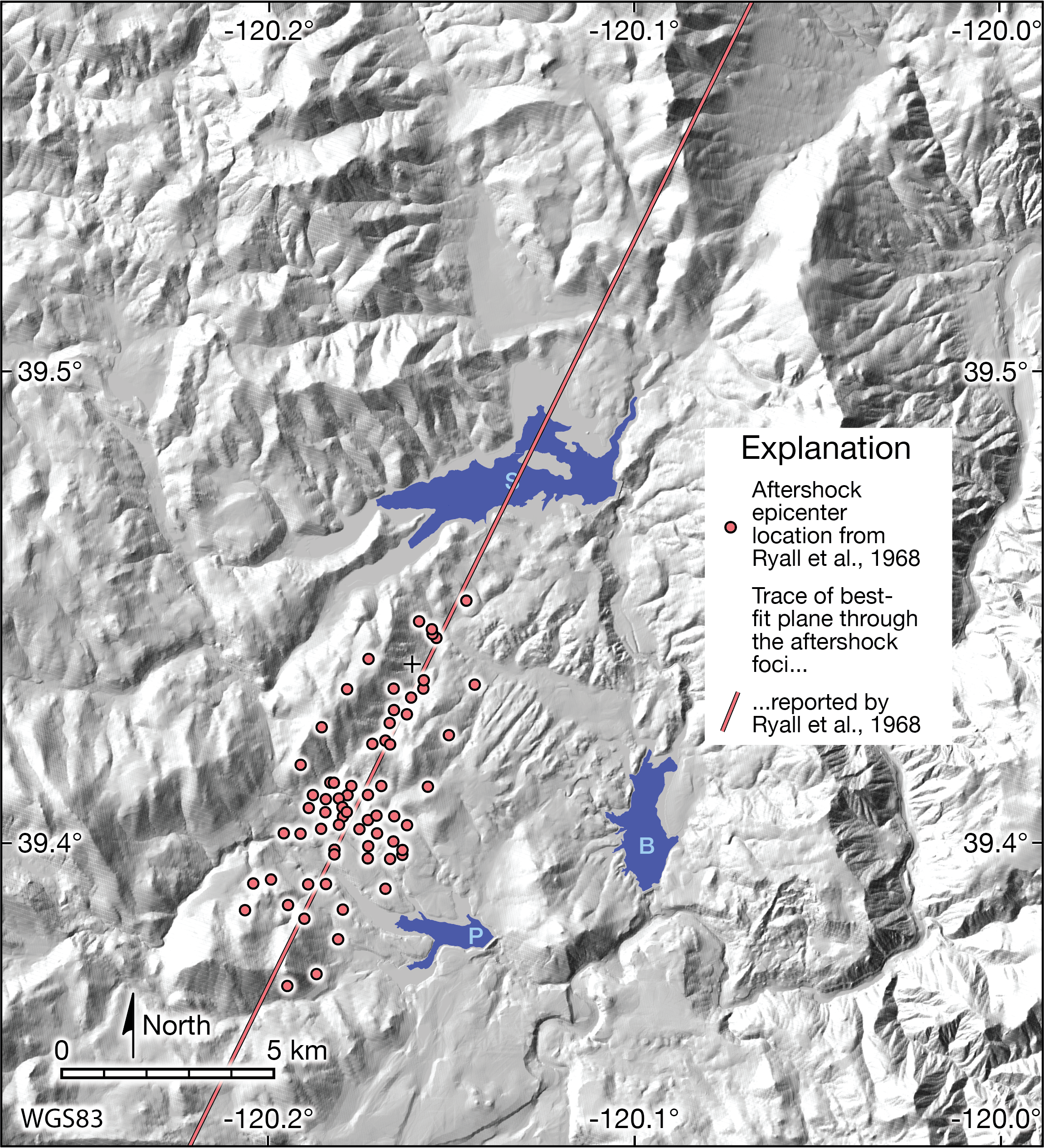
- Finished map from Adobe Illustrator file AftershocksBFPWGS83_Jan09.ai with aftershock epicenters from Ryall et alia (1968): https://croninprojects.org/Hobart/Map19_RyallAftershocks_V2.png
- Finished map from Adobe Illustrator file AftershocksBFPWGS83_Jan09.ai with aftershock epicenters from Ryall et alia (1968) and the trace of the best-fit plane through those aftershock foci: https://croninprojects.org/Hobart/Map20_RyallAftershocks&RBFP_V2.png
- Finished map from Adobe Illustrator file AftershocksBFPWGS83_Jan09.ai with aftershock epicenters from Greensfelder (1968) and Ryall et alia (1968): https://croninprojects.org/Hobart/Map21_Ryall&GreensfelderAftershocks_V2.png
- Finished map from Adobe Illustrator file AftershocksBFPWGS83_Jan09.ai with the ground-surface trace of the best-fit plane through the foci of aftershocks reported by Greensfelder (1968) and Ryall et alia (1968): https://croninprojects.org/Hobart/Map22_CompositeM-BFP_V2.png
- Finished map from Adobe Illustrator file AftershocksBFPWGS83_Jan09.ai with aftershock epicenters from Greensfelder (1968) and Ryall et alia (1968), and the trace of the best-fit plane through those aftershock foci: https://croninprojects.org/Hobart/Map23_AllAftershocks&BFP_V2.png
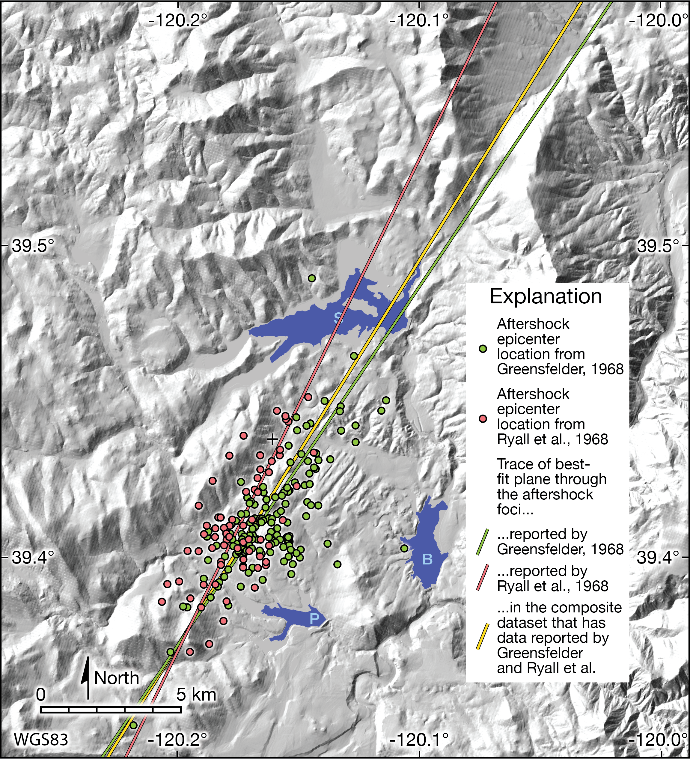
- Finished map from Adobe Illustrator file AftershocksBFPWGS83_Jan09.ai with aftershock epicenters from Greensfelder (1968) and Ryall et alia (1968), and the traces of all three best-fit planes through those three sets of aftershock foci: https://croninprojects.org/Hobart/Map24_AllAftershocks&AllBFP_V2.png
Figures for GPS Strain Analysis
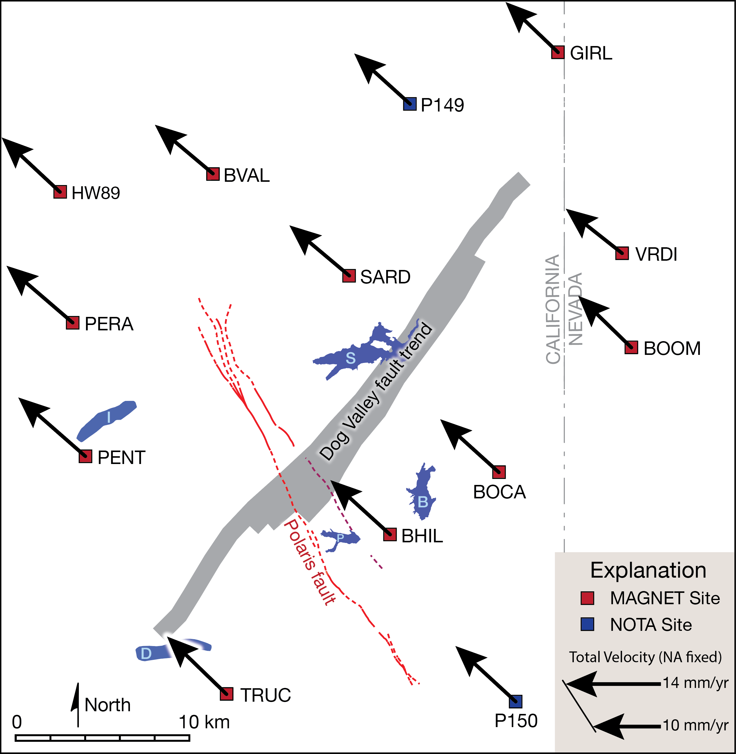
- Finished map from Adobe Illustrator file GNSS-maps-V2.ai showing the total instantaneous velocity vector for each of the GPS sites in the study area in a reference frame fixed to North America (Kreemer et al., 2014): https://croninprojects.org/Hobart/TotalSiteVel-V1.png
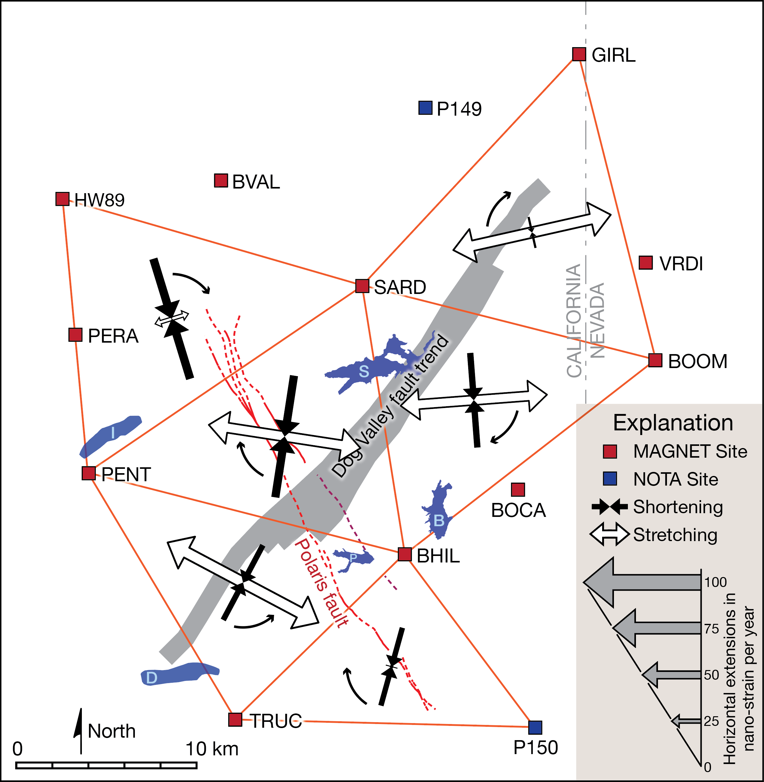
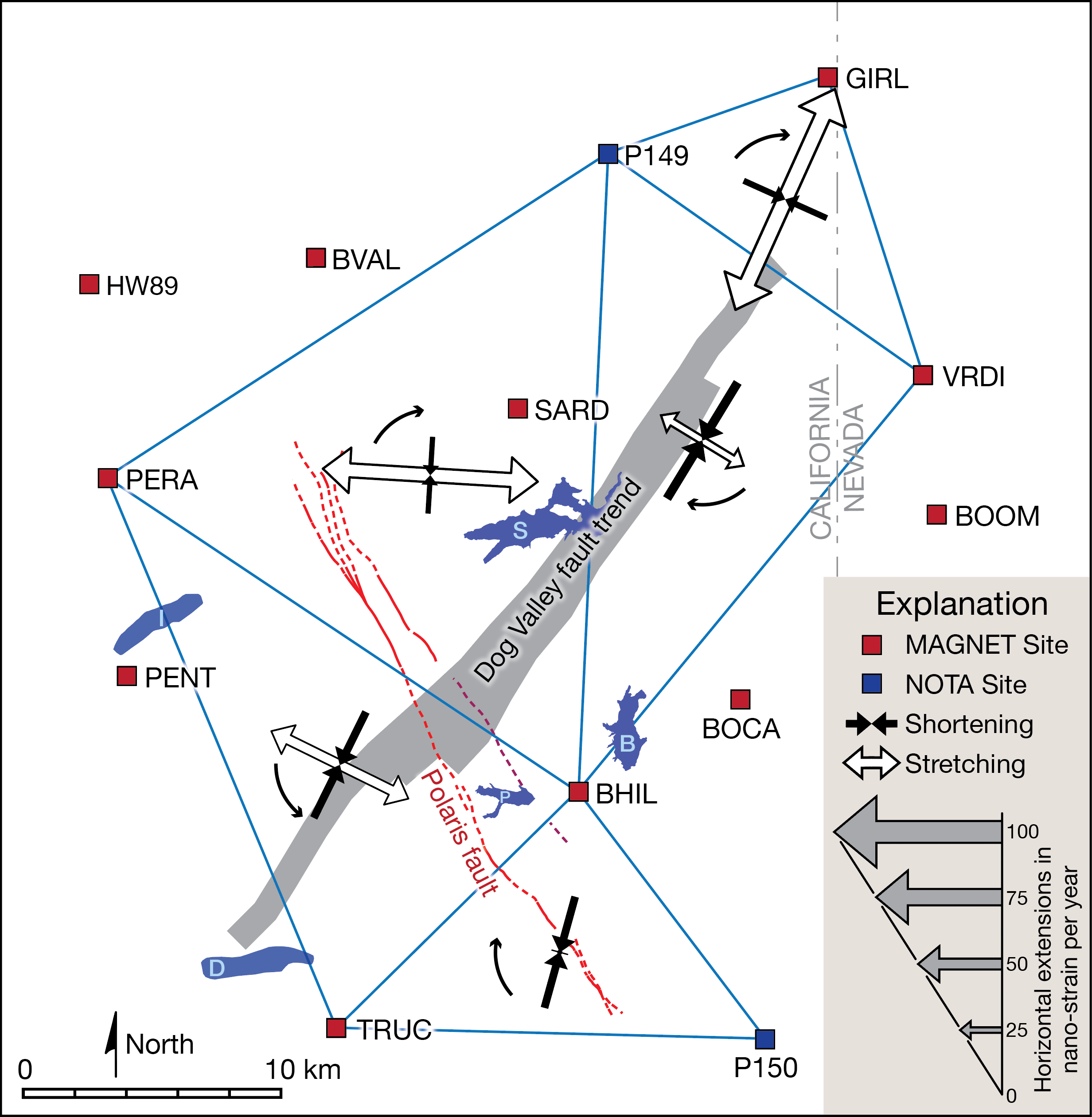
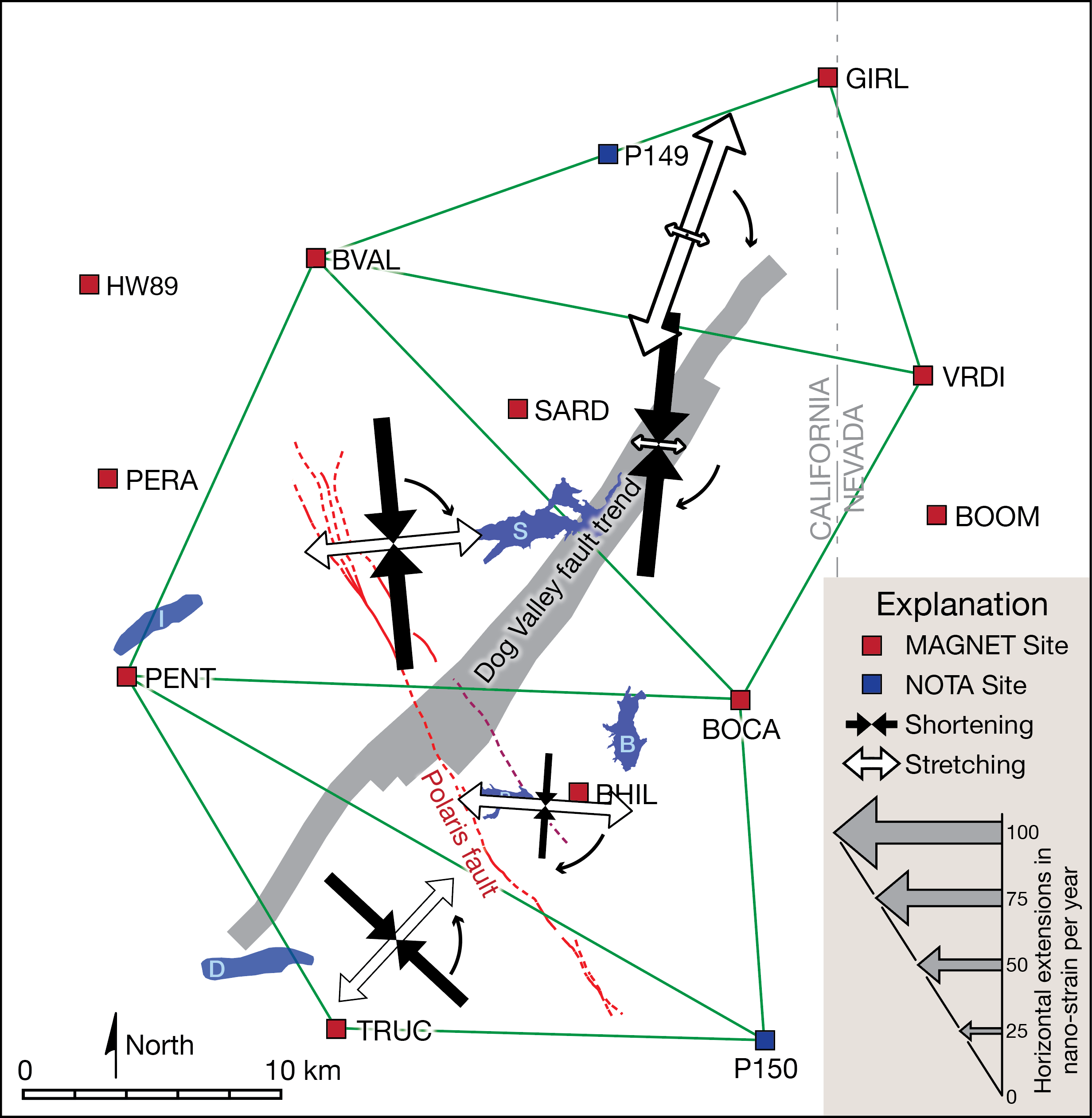
- Finished map from Adobe Illustrator file GNSS-maps-V2.ai showing crustal-strain results for the "orange" network across the Dog Valley and Polaris faults: https://croninprojects.org/Hobart/GPS-network-1-V2.png
- Finished map from Adobe Illustrator file GNSS-maps-V2.ai showing crustal-strain results for the "orange" network across the Dog Valley and Polaris faults: https://croninprojects.org/Hobart/GPS-network-2-V2.png
- Finished map from Adobe Illustrator file GNSS-maps-V2.ai showing crustal-strain results for the "orange" network across the Dog Valley and Polaris faults: https://croninprojects.org/Hobart/GPS-network-3-V2.png
GPS-Strain Analysis
Data
GPS site location and velocity data (relative to a fixed North American plate) were obtained from the Nevada Geodetic Laboratory at the University of Nevada-Reno (http://geodesy.unr.edu/NGLStationPages/gpsnetmap/GPSNetMap_MAG.html). Geodetic sites from the MAGNET and NOTA networks were used.
The process of determining crustal strain from the velocities of three noncolinear GNSS sites is explained in documents associated with the GETSI module "GPS, Strain, and Earthquakes" (https://serc.carleton.edu/getsi/teaching_materials/gps_strain/index.html). In particular, the Primer on Infinitesimal Strain Analysis in 1, 2, and 3-D (https://d32ogoqmya1dw8.cloudfront.net/files/getsi/teaching_materials/gps_strain/infinitesimal_strain_analysis_.v2.docx) and the Algorithm for Triangle-Strain Analysis (https://croninprojects.org/GETSI-EER2018/TriangleStrainAlgorithm.pdf) contain explanations for the method and an algorithm on which the analysis code is based. The analysis code is available in three forms at present:
Several videos about the use of GPS velocities for crustal-strain analysis are posted on the YouTube channel Cronin-Structure-Ed (https://www.youtube.com/channel/UCZJu-OKjQ29vJiUbmmDMMBQ). A student's brief explanation of how to interpret the strain calculator output is available via https://d32ogoqmya1dw8.cloudfront.net/files/getsi/teaching_materials/gps_strain/explanation_gps_strain_calculator.v3.pdf
(.pdf file) [
Microsoft Word .docx file
]. A strain ellipse visualization tool is available via https://d32ogoqmya1dw8.cloudfront.net/files/getsi/teaching_materials/gps_strain/strain_ellipse_visualization_t.zip. It requires a free copy of Wolfram CDF Player (
https://www.wolfram.com/cdf-player/
)
The sources for all of the raw GPS location and velocity data used in this analysis are as follows:
Data Analysis
- 1-GIRL-SARD-BOOM.xls
- 2-HW89-SARD-PENT.xls
- 3-PENT-BHIL-SARD.xls
- 4-TRUC-BHIL-PENT.xls
- 5-TRUC-P150-BHIL.xls
- 6-BHIL-BOOM-SARD.xls
- 7-TRUC-BHIL-PERA.xls
- 8-BHIL-P149-PERA.xls
- 9-BHIL-VRDE-P149.xls
- 10-GIRL-P149-VRDE.xls
- 11-GIRL-BVAL-VRDE.xls
- 12-BVAL-BOCA-VRDE.xls
- 13-PENT-BOCA-BVAL.xls
- 14-P150-BOCA-PENT.xls
- 15-PENT-TRUC-P150.xls
- Triplets-Results.xlsx
Graphics
- GNSS-maps-V2.ai (version of December 30, 2020)
- TotalSiteVel-V1.png
- GPS-network-1-V2.png
- GPS-network-2-V2.png
- GPS-network-3-V2.png
SLAM Analysis
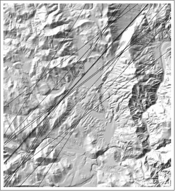
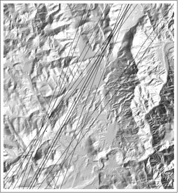
The Seismo-Lineament Analysis Method (SLAM) uses data from earthquake focal mechanism solutions to delineate an area on the ground surface (i.e., the seismo-lineament) within which the ground-surface trace of the fault that generated the earthquake would be found if the active fault surface is planar and emergent. See Cronin (2014; http://croninprojects.org/Vince/SLAM/CroninINQUA_PATA14.pdf) for more details.
The Mathematica notebooks used to define the seismo-lineaments contain some expllanations of how to run the code. For those who do not have a copy of Mathematica with which to view the native notebook, a PDF image of the code is also provided.
Mathematica notebook (code) and input-data files
Revised January 8, 2021
- SLAMcode20210103.nb, configured to read the first record of the earthquake data file. This version bases focal location on input UTM coordinates in WGS83, rather than converting from the geographic coordinate system to UTM NAD27.
The PDF image of the SLAMcode20210103..nb Mathematica notebook: SLAMcode20210103.pdf
- The earthquake datafile EQFMdata-Truckee Basin-2021Jan8.xlsx
This version of the datafile includes focal locations expressed in the UTM coordinate system in the WGS83 datum. Conversions from the original input geographic coordinates were done using the NCAT web app (https://www.ngs.noaa.gov/NCAT/index.xhtml).
- The digital elevation model, based on data digitized from USGS topographic maps at a grid spacing of ~9.35 m, expressed in a WGS83 datum (although the original topo maps that were digitized to create the DEM were created in the NAD27 datum): DogValleyFull27.dat
Note: Appending ".txt" to the ending of the digital elevation model file allows you to read the ".dat" file as a common text file.
Mapped Results
Revised January 8, 2021
The basemap is WGS83, UTM Zone 10, easting 734200mE to 759571mE, northing 4357573mN to 4385291mN, created from data obtained from the US National Elevation Dataset circa 2009. The grid convergence is 1.82467° at the center of the map area, with grid north a clockwise rotation from true north.
The graphics file with the coarse-resolution basemap, geographic coordinates, scale, and north arrow is accessible via https://CroninProjects.org/Hobart/Basemap2021Jan4.ai
The graphics file for all of the finished graphics referenced below is accessible via https://CroninProjects.org/Hobart/SLAMresults-2021Jan5.ai. You might need to right-click or (for Macintosh) control-click on the link to download.
- Basemap plus focal mechanism for 1966 M6 earthquake, from Adobe Illustrator document SLAMresults-2021Jan5.ai: Map01_1966EQFM_2021Jan08.png
- Basemap, focal mechanism, and seismo-lineament for 1966 M6 earthquake, from Adobe Illustrator document SLAMresults-2021Jan5.ai: Map02_1966EQFMSL_2021Jan08.png
Raw SLAM output for this event: 1966EQ-SeisLinOutput-01042021.jpg
- Basemap plus focal mechanism for 1977 earthquake, from Adobe Illustrator document SLAMresults-2021Jan5.ai: Map03_1977EQFM_2021Jan08.png
- Basemap, focal mechanism, and seismo-lineament for 1977 earthquake, from Adobe Illustrator document SLAMresults-2021Jan5.ai: Map04_1977EQFMSL_2021Jan08.png
Raw SLAM output for this event: 1977EQ-SeisLinOutput-01042021.jpg
- Basemap plus focal mechanism for 1983 earthquake, from Adobe Illustrator document SLAMresults-2021Jan5.ai: Map05_1983EQFM_2021Jan08.png
- Basemap, focal mechanism, and seismo-lineament for 1983 earthquake, from Adobe Illustrator document SLAMresults-2021Jan5.ai: Map06_1983EQFMSL_2021Jan08.png
Raw SLAM output for this event: 1983EQ-SeisLinOutput-01042021.jpg
- Basemap plus focal mechanism for 2004 earthquake (21370352), from Adobe Illustrator document SLAMresults-2021Jan5.ai: Map07_2004EQFM_2021Jan08.png
- Basemap, focal mechanism, and seismo-lineament for 2004 earthquake (21370352), from Adobe Illustrator document SLAMresults-2021Jan5.ai: Map08_2004EQFMSL_2021Jan08.png
Raw SLAM output for this event: 2004061214EQ-SeisLinOutput-01042021.jpg
- Basemap plus focal mechanism for 2004 earthquake (21370353), from Adobe Illustrator document SLAMresults-2021Jan5.ai: Map09_2004EQFM_2021Jan08.png
- Basemap, focal mechanism, and seismo-lineament for 2004 earthquake (21370353), from Adobe Illustrator document SLAMresults-2021Jan5.ai: Map10_2004EQFMSL_2021Jan08.png
Raw SLAM output for this event: 2004161215EQ-SeisLinOutput-01042021.jpg
- Basemap plus focal mechanisms for 1966. 1977, 1983, and 2004 (21370352) earthquakes, from Adobe Illustrator document SLAMresults-2021Jan5.ai: Map11_FourEQFM_2021Jan08.png
- Basemap, focal mechanisms, and seismo-lineaments for 1966. 1977, 1983, and 2004 (21370352) earthquakes, from Adobe Illustrator document SLAMresults-2021Jan5.ai: Map12_FourEQFMSL_2021Jan08.png
- Basemap, focal mechanisms for 1966. 1977, 1983, and 2004 (21370352) earthquakes, and aftershock epicenters, from Adobe Illustrator document SLAMresults-2021Jan5.ai: Map13_aftershocksAndFourEQFM_2021Jan08.png
- Basemap, aftershock epicenters, focal mechanisms and seismo-lineaments for 1966. 1977, 1983, and 2004 (21370352) earthquakes, from Adobe Illustrator document SLAMresults-2021Jan5.ai: Map14_aftershocksAndFourEQFMSL_2021Jan08.png
- Basemap, focal mechanisms for 1966. 1977, 1983, and 2004 (21370352) earthquakes, aftershock epicenters, and trace of best-fit plane through the aftershocks, from Adobe Illustrator document SLAMresults-2021Jan5.ai: Map15_aftershocksBFP_FourEQFM_2021Jan08.png
- Basemap, aftershock epicenters, focal mechanisms and seismo-lineaments for 1966. 1977, 1983, and 2004 (21370352) earthquakes, and trace of best-fit plane through the aftershocks, from Adobe Illustrator document SLAMresults-2021Jan5.ai: Map16_aftershocksBFP_FourEQFMSL_2021Jan08.png
Best-Fit Plane Analysis
Best-Fit-Plane Codes, revised December 23, 2020
The codes listed below were all written in Mathematica and are raw research codes based on the published code by Paláncz et al (2013). Contact Vince Cronin for clarification about their use and contents. You might need to right-click or control-click to download the Mathematica notebook code.
- Best-fit plane through aftershock hypocenter location data published by Greensfelder (1968)*: croninprojects.org/Hobart/GreensfelderBFPcode.nb
- Best-fit plane through aftershock hypocenter location data published by Ryall et al (1968): croninprojects.org/Hobart/RyallBFPcode.nb
- Best-fit plane through a composite dataset including aftershock hypocenter location data published by Greensfelder (1968)* and Ryall et al (1968), using the mean location for co-reported events: croninprojects.org/Hobart/CompositeBFPcode.nb
*Spatial outliers (Greensfelder events 70 and 91) and events not recorded by the local-area network (1-12 and 116) were excluded.
Modified SLAM Codes Used in the Best-Fit-Plane Analysis, revised December 23, 2020
The codes listed below were all written in Mathematica and are raw research codes. Contact Vince Cronin for clarification about their use and contents. You might need to right-click or control-click to download the Mathematica notebook code.
To produce their results, they called on the following datafiles
- croninprojects.org/Hobart/SLAMGreensfelder21Dec2020.nb
- croninprojects.org/Hobart/SLAMRyall21Dec2020.nb
- croninprojects.org/Hobart/SLAMComposite-21Dec2020.nb
Mapped Results, revised January 9, 2021
The following map graphics were produced using modified SLAM codes acting on [1] an Excel dataset that contains results of the best-fit plane analysis, and [2] a DEM dataset with a node spacing of about 9.3 meters. All are preliminary results that are subject to revision, and are © 2020-2021 by the authors.
Graphics datafile for aftershocks and best-fit plane analysis: https://CroninProjects.org/Hobart/AftershocksBFPWGS83_Jan09.ai
- Finished map from Adobe Illustrator file AftershocksBFPWGS83_Jan09.ai with aftershock epicenters from Greensfelder (1968): https://croninprojects.org/Hobart/Map17_GreensfelderAftershocks_V2.png
- Finished map from Adobe Illustrator file AftershocksBFPWGS83_Jan09.ai with aftershock epicenters from Greensfelder (1968) and the trace of the best-fit plane through those aftershock foci: https://croninprojects.org/Hobart/Map18_GreensfelderAftershocks&GBFP_V2.png
- Finished map from Adobe Illustrator file AftershocksBFPWGS83_Jan09.ai with aftershock epicenters from Ryall et alia (1968): https://croninprojects.org/Hobart/Map19_RyallAftershocks_V2.png
- Finished map from Adobe Illustrator file AftershocksBFPWGS83_Jan09.ai with aftershock epicenters from Ryall et alia (1968) and the trace of the best-fit plane through those aftershock foci: https://croninprojects.org/Hobart/Map20_RyallAftershocks&RBFP_V2.png
- Finished map from Adobe Illustrator file AftershocksBFPWGS83_Jan09.ai with aftershock epicenters from Greensfelder (1968) and Ryall et alia (1968): https://croninprojects.org/Hobart/Map21_Ryall&GreensfelderAftershocks_V2.png
- Finished map from Adobe Illustrator file AftershocksBFPWGS83_Jan09.ai with the ground-surface trace of the best-fit plane through the foci of aftershocks reported by Greensfelder (1968) and Ryall et alia (1968): https://croninprojects.org/Hobart/Map22_CompositeM-BFP_V2.png
- Finished map from Adobe Illustrator file AftershocksBFPWGS83_Jan09.ai with aftershock epicenters from Greensfelder (1968) and Ryall et alia (1968), and the trace of the best-fit plane through those aftershock foci: https://croninprojects.org/Hobart/Map23_AllAftershocks&BFP_V2.png
- Finished map from Adobe Illustrator file AftershocksBFPWGS83_Jan09.ai with aftershock epicenters from Greensfelder (1968) and Ryall et alia (1968), and the traces of all three best-fit planes through those three sets of aftershock foci: https://croninprojects.org/Hobart/Map24_AllAftershocks&AllBFP_V2.png
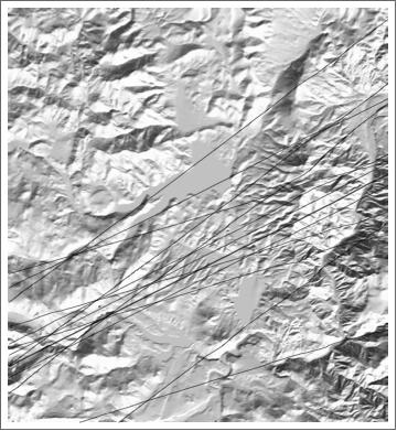
- Bare-Earth image of basemap: croninprojects.org/Hobart/BareEarthHillshade.pdf
-->
*Spatial outliers (events 70 & 91) and events not recorded by the local-area network (1-12 & 116) were excluded.
Aftershock Hypocenter Location Datasets Used in the Best-Fit-Plane Analysis
- From Greensfelder (1968)*: https://croninprojects.org/Hobart/GreenEQAfterNAD83UTMzone10N-rev.csv
- From Ryall et al. (1968): https://croninprojects.org/Hobart/RyallEQAfterNAD83UTMzone10N.csv
- Composite dataset derived from Greensfelder (1968)* and Ryall et al. (1968), using the mean location for co-reported events: https://croninprojects.org/Hobart/CompositeNAD83UTMZone10N.csv
- Composite dataset derived from Greensfelder (1968)* and Ryall et al. (1968), using Greensfelder data for co-reported events: https://croninprojects.org/Hobart/CompositeG-NAD83UTMZone10N.csv
- Composite dataset derived from Greensfelder (1968)* and Ryall et al. (1968), using Ryall et al data for co-reported events: https://croninprojects.org/Hobart/CompositeR-NAD83UTMZone10N.csv
*Spatial outliers (Greensfelder events 70 and 91) and events not recorded by the local-area network (1-12 and 116) were excluded.
References and Selected Bibliography
- Ashburn, J.A., 2015, Investigation of a lineament that might mark the ground-surface trace of the Dog Valley Fault, Truckee area, northern California: Baylor University, B.S. thesis, available via http://CroninProjects.org/Vince/AshburnBSThesis2015.pdf.
- Bryant, W.A., compiler, 2017, Fault number 27, Dog Valley fault zone, in Quaternary fault and fold database of the United States: U.S. Geological Survey website, https://earthquakes.usgs.gov/hazards/qfaults, accessed 10/12/2020 10:43 AM; Accessed via https://earthquake.usgs.gov/cfusion/qfault/show_report_AB_archive.cfm?fault_id=27§ion_id=
- Cronin, V.S., 2014, Seismo-Lineament Analysis Method (SLAM), using earthquake focal mechanisms to help recognize seismogenic faults: Proceedings of the 5th International INQUA meeting on Paleoseismology, Active Tectonics and Archeoseismology (PATA Days), 21-27 September, Busan, South Korea, p. 21-27 September 2014, p. 28-31, ISBN 9791195344109 93450; available via http://croninprojects.org/Vince/SLAM/CroninINQUA_PATA14.pdf.
- Cronin, V.S., Millard, M., Seidman, L., and Bayliss, B., 2008, The Seismo-Lineament Analysis Method (SLAM) -- A reconnaissance tool to help find seismogenic faults: Environmental and Engineering Geology, v. 14, no. 3, p. 199-219. Available via http://eeg.geoscienceworld.org/cgi/content/abstract/14/3/199.
- Greensfelder, R., 1968, Aftershocks of the Truckee, California earthquake of September 12, 1966: Bulletin of the Seismological Society of America, v. 58, no. 5, p. 1607- 1620.
- Grose, T.L.T., 2000, Geologic map of the Loyalton 15-minute quadrangle, Lassen, Plumas, and Sierra counties, California: California Division of Mines and Geology Open-File Report OFR 00-25, map scale 1:62,500.
- Hawkins, F.F., LaForge, R. and Hansen, R.A., 1986, Seismotectonic study of the Truckee/Lake Tahoe area northeastern Sierra Nevada, California for Stampede, Prosser Creek, Boca, and Lake Tahoe dams: U.S. Bureau of Reclamation Seismotectonic Report No. 85-4, 210 p.
- Hunter, L.E., Howle, J.F., Rose, R.S., and Bawden, G.W., 2011, LiDAR-assisted identification of an active fault near Truckee, California: Bulletin of the Seismological Society of America, v. 101, no. 3, p., 1162-1181, doi:10.1785/0120090261.
- Jennings, C.W., 1994, Fault activity map of California and adjacent areas, with locations of recent volcanic eruptions: California Division of Mines and Geology Geologic Data Map 6, 92 p., 2 pls., scale 1:750,000.
- Kachadoorian, R., Yerkes, R.F., and Waananen, A.O., 1967, Effects of the Truckee, California, earthquake of September 12, 1966: U.S. Geological Survey, Circular 573, p. 14.
- Kreemer, C., Blewitt, G., Klein, E.C., 2014, A geodetic plate motion and Global Strain Rate Model: Geochemistry, Geophysics, Geosystems, v. 15, p. 3849-3889, doi:10.1002/2014GC005407.
- Lindsay, R., 2012, Seismo-lineament analysis of selected earthquakes in the Tahoe-Truckee area, California and Nevada: Baylor University, M.S. thesis, available via https://baylor-ir.tdl.org/baylor-ir/handle/2104/8441.
- NCALM, 2014, Full waveform LiDAR survey of Tahoe National Forest: available via http://opentopo.sdsc.edu/raster?opentopoID=OTSDEM.032017.26910.2
- NCEDC, 2017, Northern California earthquake data center: available via http://quake.geo.berkeley.edu/ncedc/catalog-search.html.
- OpenTopography.org, 2020, 2014 USFS Tahoe National Forest Lidar, 1-m DEM, https://doi.org/10.5069/G9V122Q1
- Paláncz, B., Lovas, T., Molnár, B., 2013, Plane fitting to point cloud via Gröbner basis: Wolfram Library Archive, accessed 2020 Nov. 2 via https://library.wolfram.com/infocenter/ID/8769/
- Reed, T.H., 2014, Spatial correlation of earthquakes with two known and two suspected seismogenic faults, north Tahoe-Truckee area, California: Baylor University, M.S. thesis, available via https://baylor-ir.tdl.org/baylor-ir/handle/2104/9097.
- Ryall, A., Van Wormer, J.D., and Jones, A.J., 1968, Triggering of micro-earthquakes by earth tides, and other features of the Truckee, California, earthquake sequence of September, 1966: Bulletin of the Seismological Society of America, v. 58, no. 1, p. 215-248.
- Strasser, M.P., 2017, Spatial correlation of selected earthquakes with the Dog Vally Fault in northern California using LiDAR and GPS data: MS thesis, Baylor University, accessible via http://croninprojects.org/Strasser/Matthew_Strasser_Masters.pdf
- Tsai, Y-B., and Aki, K., 1970, Source mechanism of the Truckee, California earthquake of September 12, 1966: Bulletin of the Seismological Society of America. v. 60, no. 4, p. 1199-1208.
- USACE, 2008, SPK_20080922-26: accessed September 2016 via https://griduc.rsgis.erdc.dren.mil/
- USBR, 2011, Draft Environmental Assessment, Stampede Dam Safety of Dams Modification: U.S. Bureau of Reclamation, available via https://www.usbr.gov/mp/nepa/includes/documentShow.php?Doc_ID=8623.
- USBR, 2012, Stampede Dam safety of dams modification: U.S. Bureau of Reclamation, available via https://www.usbr.gov/mp/nepa/includes/documentShow.php?Doc_ID=9930 and https://www.usbr.gov/mp/nepa/nepa_project_details.php?Project_ID=8182.
- USGS, 2016, National elevation dataset: accessed April 2016, available via http://ned.usgs.gov.
- USGS, 2017, Quaternary fault and fold database of the United States: available via http://earthquake.usgs.gov/hazards/qfaults/.
- Waldhauser, F., 2017, Real-time double-difference earthquake locations for northern California, available via http://ddrt.ldeo.columbia.edu.
If you have any questions or comments about this site or its contents, drop an email to the humble
webmaster
.
All of the original content of this website is © 2020-2021 by Vincent S. Cronin or Kate Hobart
